Flood Estimation [GATE Notes]

What is the Flood Estimation?

Flood estimation is one of the topics of engineering hydrology in which analysis of floods will be carried out. Flood estimation will be carried out based on the precipitation occurring in the catchment. Flood analysis is required to know the prevailing flood conditions for a particular catchment basin.

The estimation of flood analysis can be done based on various methods, including theoretical and analytical methods. These methods of flood analysis are important for the GATE CE exam and will be explained in this article.

Flood-Peak Estimation

A flood is an unusually high stage in a river, usually the level at which the river overflows its banks and inundates the adjoining area. The design of bridges, culvert waterways, and spillways for dams and the estimation of the score at a hydraulic structure are some examples wherein flood-peak values are required. To estimate the magnitude of a flood peak, the following alternative methods are available:

1. Rational method
2. Empirical method
3. unit-hydrograph technique
4. Flood-frequency studies

Rational Method

The most realistic way to use the Rational Method is to consider it as a statistical link between rainfall frequency distribution and runoff. As such, it provides a means of estimating the design flood of a certain return period, with the rainfall duration equal to the concentration time.

If t_p ≥ t_c

Q_p = (1/36) k P_c A

Where, 

• Q_p = Peak discharge in m³/sec
• P_C = Critical design rainfall in cm/hr
• A = Area catchment in hectares
• K = Coefficient of runoff.
• t_D = Duration of rainfall
• t_C = Time of concentration

Empirical Formulae

(a) Dickens Formula (1865)

Q_p = C_D A^3/4

Where,

• Q_p = Flood peak discharge in m³/sec
• A = Catchment area in km².
• C_D = Dickens constant, 6 ≤ C_D ≤ 30.

(b) Ryes formula (1884)

Q_p = C_R A^2/3

Where,

• C_R = Ryes constant
• = 8.8 for the constant area within 80 km from the cost.
• = 8.5 if the distance of area is 80 km to 160 km from the cost.
• = 10.2 if the area is Hilley and away from the cost.

(c) Inglis Formula (1930)

Where

• A = Catchment area in Km².
• Q_P = Peak discharge in m³/sec.

Flood Frequency Studies

Flood frequency analysis will be carried out to know the frequency of a particular flood that occurs at a certain interval. These analyses will be based on the different parameters, which will be explained below.

(i) Recurrence interval or return Period

T = 1/P
where, P = Probability of occurrence

(ii) Probability if non-occurrence: q = 1-P

(iii) Probability of an event occurring r times in ‘n’ successive years: = ⁿC_r x p^r x q^n-r

 ⁿC_r = n! /(n-r)r!

(iv) Reliability: (probability of non-occurrence /Assurance) = qⁿ

(v) Risk = 1-qⁿ = 1-(1-P)ⁿ

(vi) Safety Factor = Design values of hydrological parameter adopted / Estimated value of the hydrological parameter

(vii) Safety Margin = Design value of the hydrological parameter – Estimated value of the hydrological parameter

Gumbel’s Method in Flood Estimation

The extreme value distribution was an introduction by Gumbel (1941) and is commonly known as Gumbel’s distribution. It is one of the most widely used probability distribution functions for extreme values in hydrologic and meteorologic studies for predicting flood peaks, maximum rainfall, and maximum wind speed.

Gumbel defined a flood as the largest of the 365 daily flows, and the annual series of flood flows constitute a series of the largest values of flows.

Based on the probability distribution.

(i) X_T =X‾ + Kσ

Where 

• X_T = Peak value of hydrologic data
• K = Frequency factor

 

y_T = Reduced variate

• T = Recurrence interval in year
• y_n = Reduced mean = 0.577
• S_n = Reduced standard deviation.
• S_n = 1.2825 for N → ∞

Confidence Limit in Flood Estimation

Since the value of the variate for a given return period, x_T is determined by Gumbel’s method. Which can have errors due to the limited sample data used. An estimate of the confidence limits of the estimates is desirable. The confidence interval indicates the limits to the calculated value between which the true value can lie with specific probability based on sampling errors only.

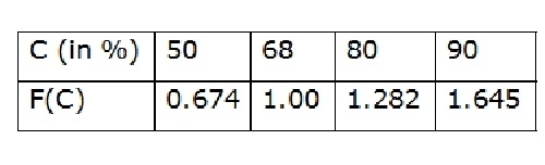
For a confidence probability c, the confidence interval of the variate x_T is bounded by values x₁ and x₂ given by

X₂/X₁ = X_T ± f(c).S_e

Where f(c) is a confidence probability ‘C’ function. It can be represented as below.

S_e = Probability error

Where,

• N = Sample size
• B = factor
• σ = Standard deviation

Important Topics for Gate Exam
Non-Newtonian Fluids	Open Loop Control System
Pattern Allowances	Poissons Ratio
Pressure Measurement	Prestressed Concrete
Prestressing Systems	Principle of Conservation of Energy
Properties of Aggregate	Properties of Concrete