Round Robin Scheduling

What is Round Robin Scheduling?

The round robin scheduling is a preemptive FCFS based on a timeout interval (quantum or time slice). A running process is preempted (interrupted) by the clock, and the process will be kept in the ready state and then submits a process from the ready queue into the CPU.

In the round robin scheduling algorithm, if the time quantum of the process is shorter, it leads to more context switches (overhead). If the time quantum of the process is substantial (time quantum greater than every process service time), then the round robin scheduling algorithm will work the same as FCFS.

Flowchart of Round Robin Scheduling Algorithm

The flowchart of the round robin scheduling algorithm is given below. In this, all the processes are in the ready queue. The burst time of every process is compared to the time quantum.

If the burst time of the process is less than the time quantum in the round robin scheduling algorithm, the process is executed to its burst time. Else, the process is executed upto the time quantum, and when the time quantum expires, it checks if the process is executed completely and then terminates. Else, it goes again to the ready queue.

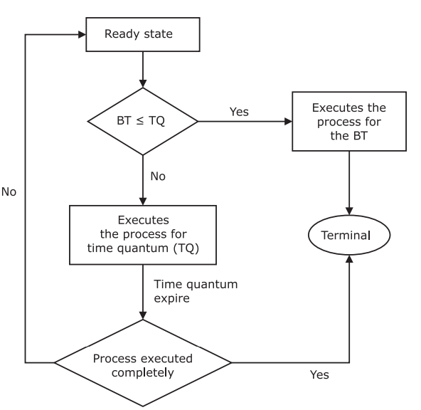
Figure: Flowchart of Round Robin Scheduling Algorithm

Advantages of Round Robin Scheduling

The advantage of the round robin scheduling algorithm is fairness since every process in the ready state or queue gets an equal time quantum or the CPU share.

The round robin scheduling algorithm is simple to implement. The newly created process is added to the end of the ready queue, and the round robin scheduling algorithm does not suffer starvation.

Download Formulas for GATE Computer Science Engineering - Discrete Mathematics

Disadvantages of Round Robin Scheduling

The disadvantage of the round robin scheduling is that this algorithm gives a larger waiting time for the process and the response time of the process is also very large compared to other scheduling algorithms.

The round robin scheduling algorithm provides a low throughput of the system because there are more context switches in the round robin scheduling algorithm, which increase the overhead of the CPU.

Download Formulas for GATE Computer Science Engineering - Algorithms

Round Robin Scheduling Example 

Consider the following 5 processes: A, B, C, D, and E, with arrival time and burst time as given below:

What are the average waiting and turnaround times for the round robin scheduling algorithm(RR) with a time quantum of 2?

For the round-robin scheduling algorithm, we have the ready queue as:

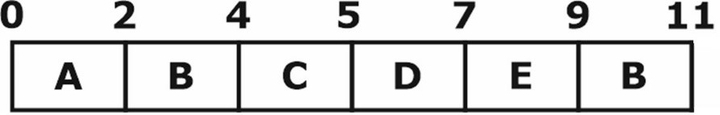
A, B, C, D, E, B, E, B

The Gantt chart using the RR algorithm is as follows.

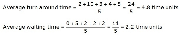
Now, we know

• Turnaround time = Completion time – Arrival time
• Waiting time = Turnaround time – Burst time

Now,