- Home/
- GATE ELECTRICAL/
- GATE EE/
- Article
What is Laplace Transform?
By BYJU'S Exam Prep
Updated on: September 25th, 2023

Laplace Transform is one of the most significant mathematic tools that found extensive application in various forms of engineering. The French mathematician “Pierre Simon De Laplace” first used a transform similar to this in his work on the “Probability Theory” then, these transforms are populated with the name “Laplace Transforms”.
Here we will provide the tabulated formulas of the Laplace transforms of some general mathematical functions along with the definition of Laplace transforms, then we will discuss further the significance, and various properties of Laplace transforms.
Table of content
What is the Laplace Transform?
The Laplace Transform is a useful tool for analyzing any electrical circuit, which we can convert from the Integral-Differential Equations to Algebraic Equations by replacing the original variables with new ones representing their Integral and Derivative counterpart.
In engineering, simulation, and design are the crucial stages in the physical realization of any invention because one cannot afford the trial-and-error method on a complex engineering project. To facilitate the design and simulation we must go through various mathematical equations. Every time it is not feasible to solve them in the time domain, especially the differential equations. To make this simple we convert these complex time-domain equations into the frequency domain where they will be simply solvable algebraic functions. In simple words, the Laplace Transform will function as a translator for the foreign tourist.
Laplace Transform Formula
If f(t) is a function of time that is defined for all values of ‘t’, then Laplace transform of 𝑓(𝑡) denoted by ℒ{𝑓(𝑡)} is defined as
ℒ{𝑓(𝑡)}=∞∫0𝑒−𝑠𝑡𝑓(𝑡)𝑑𝑡
given that the integral exists.
Where ‘s’ is a real or complex number and ′ℒ′ is the Laplace transformation operator. Since ℒ{𝑓(𝑡)} is a function of ‘s’ this can be written as F(s).
i.e., ℒ{𝑓(𝑡)}=𝐹(𝑠) which can also be written as 𝑓(𝑡)=ℒ−1{𝐹(𝑠)}, then 𝑓(𝑡) is called as “Inverse Laplace Transform” of F(s).
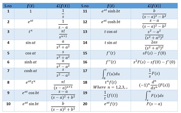
Laplace Transform Table
Significance of Laplace Transform
Laplace Transform is significant in the analysis of continuous-time signals and systems in various aspects like frequency domain analysis, damping and frequency characterization of continuous-time signals, transfer function characterization of continuous-time LTI systems, stability, and steady-state analysis in control systems, eigenfunction of LTI systems, etc.
Here we will discuss the importance of the Laplace Transform in certain aspects of continuous timeous-time signals and systems.
Transfer Function
The transfer function of a system is the ratio of the Laplace transform of the output to the Laplace transform of the input of that system. The location of poles and zeros of the transfer function is crucial in determining the dynamic characteristics of the system. The transfer function can unify the convolution integral and differential equation representation of a system.
Damping and frequency of a continuous signal
The growth and decay of the signal (damping) and its repetitive nature (frequency) in the time domain can be determined by using the location of poles and zeros of the Laplace transform of the concerned signal.
Transient and steady states-time analysis
The continuous-time systems can be analyzed effectively with the help of Laplace Transform. Certain characteristics such as stability, transient, and steady-state analysis can be effectively studied using Laplace Transform, hence the Laplace transform is a prominent tool in the control theory.
Fourier Transform
Since the Laplace transform requires integration over an infinite domain it is necessary to check whether it will converge or not. It is also known as the region of convergence (ROC) in the s-plane composed of damping (𝜎) and frequency (𝜔). If the ROC includes the 𝑗𝜔 axis of the s-plane, the Laplace transform of the signal coincides with the Fourier transform of the signal. So, we can find the Fourier transform of the large class of signals by using their Laplace transform. Subtly Fourier series representation of continuous-time periodic signals has a connection with the Laplace transform, this helps in reducing the computational complexity of the Fourier series by eliminating the integration.
What is the Two-Sided Laplace Transform?
Due to the significant application of causal signals (has no existence at t<0) and causal systems (zero impulse response at t<0) the Laplace transform is typically a one-sided transform, but the two-sided Laplace transform also exists. It is the Laplace transform applied to two different signals and systems. By separating the signal into its causal and anti-causal forms we can apply the one-sided Laplace transform, but care should be taken while applying the inverse Laplace Transform to get the correct signal.
The two-sided Laplace transform of a continuous-time function f(t) is
ℒ{𝑓(𝑡)}=∞∫−∞𝑒−𝑠𝑡𝑓(𝑡)𝑑𝑡 𝑠∈𝑅𝑂𝐶
Where 𝑠 = 𝜎+𝑗𝜔, and ROC is the region of convergence.
Properties of the Laplace Transform
Here we will discuss the basic properties of the Laplace Transform such as linearity, differentiation, integration, time-shifting, and convolution integral properties of the Laplace transform. Applying these Laplace Transform properties will reduce the time of calculation and will help reach the result quickly.
Property of Linearity
If F(s) and G(s) are the Laplace Transform of two signals f(t) and g(t) respectively, ‘x’ and ‘y’ are two constant values then ℒ{𝑥𝑓(𝑡)+𝑦𝑔(𝑡)}=𝑥𝐹(𝑠)+𝑦𝐺(𝑠)
Property of Differentiation:
If F(s) is the Laplace transform of the signal, then one-sided Laplace Transform its 𝑛𝑡ℎ order derivative 𝑓𝑛(𝑡) is ℒ{𝑓𝑛(𝑡)}=𝑠𝑛𝐹(𝑠)−𝑠𝑛-1𝑓(0)−𝑠𝑛-2𝑓′(0)−⋯𝑓𝑛-1(0)
If n=1, ℒ{𝑓1(𝑡)}=𝑠𝐹(𝑠)−𝑓(0)
If n=2, ℒ{𝑓2(𝑡)}=𝑠2𝐹(𝑠)−𝑠𝑓(0)−𝑓′(0)
Property of Integration
Laplace transform of the integral of a causal signal f(t) is
t∫0𝑓(𝑥)𝑑𝑥𝑡0 𝑢(𝑡)=𝐹(𝑠)/𝑠
Time-shifting property
If F(s) is the Laplace transform of the signal f(t)u(t), then the Laplace transform of the time-shifted signal 𝑓(𝑡−𝑎)𝑢(𝑡−𝑎) is,
ℒ{𝑓(𝑡−𝑎)𝑢(𝑡−𝑎)}=𝑒−𝑎𝑠𝐹(𝑠)
Property of Convolution Integral
If F(s) is the Laplace transform of the causal signal f(t), and H(s) is Laplace transform of its impulse response, then the Laplace transform of the convolution integral of 𝑓(𝑡) with ℎ(𝑡) is
ℒ{(𝑓∗ℎ)(𝑡)}=𝐹(𝑠)𝐻(𝑠).
These are some basic concepts involving the Laplace Transform, there are a lot of things that are to be discussed, and we may have a further emphasis in our lectures.
Laplace Transform of Standard Functions
The Laplace Transform of standard functions can be used to efficiently solve complex equations. Check out the Laplace Transform of standard functions provided below.


| Important Topics for Gate Exam | |
| Feedback Amplifier | Fermi Level |
| Floating Point Representation | Flow Measurement |
| Fluid Pressure | Fluid Properties |
| Flywheel | Full Subtractor |
| Gear Train | Incidence Matrix |
Get complete information about the GATE exam pattern, cut-off, and all those related things on the BYJU’S Exam Prep official youtube channel.