Linear Time Invariant System (LTI System)

What is Linear Time Invariant System (LTI System)?

The LTI system is one of the important topics of the GATE Exam. Linear time-invariant systems are a class of systems used in signals and systems that are both linear and time-invariant. Linear systems are systems whose outputs for a linear combination of inputs are the same as a linear combination of individual responses to those inputs. Time-invariant systems are systems where the output does not depend on when input was applied.

LTI systems have the property that the output is linearly related to the input. Changing the input in a linear way will change the output in the same linear way. So if the input x₁(t) produces the output y₁(t) and the input x₂(t) produces the output y₂(t), then linear combinations of those inputs will produce linear combinations of those outputs. The input {x₁(t)+x₂(t)} will produce the output {y₁(t)+y₂(t)}. Further, the input {a₁x₁(t)+a₂x₂(t)} will produce the output {a₁y₁(t)+a₂y₂(t)} for some constants a₁ and a₂.

In other words, for a system T over time t, composed of signals x₁(t) and x₂(t) with outputs y₁(t) and y₂(t)

T[a₁x₁(t) + a₂x₂(t)] = a₁T[x₁(t)] + a₂T[x₂(t)] = a₁y₁(t) + a₂y₂(t)

Homogeneity Principle

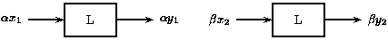
Position Principle

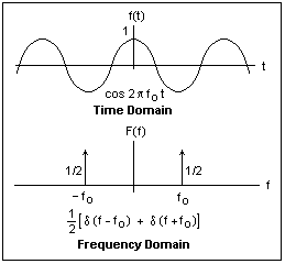
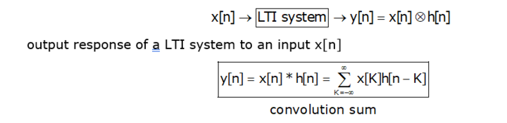
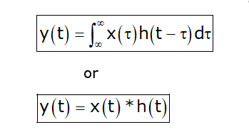
Thus, an LTI system can be described by a single function called its impulse response. This function exists in the time domain of the system. For an arbitrary input, the output of an LTI system is the convolution of the input signal with the system’s impulse response.

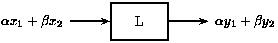
Conversely, the LTI system can also be described by its transfer function. The transfer function is the Laplace transform of the impulse response. This transformation changes the function from the time domain to the frequency domain. This transformation is important because it turns differential equations into algebraic equations, and turns convolution into multiplication.

In the frequency domain, the output is the product of the transfer function with the transformed input. The shift from time to frequency is illustrated in the following image:

Homogeneity and shift invariance may, at first, sound a bit abstract but they are very useful. To characterize a shift-invariant linear system, we need to measure only one thing: the way
the system responds to a unit impulse. This response is called the impulse response function of the system. Once we’ve measured this function, we can (in principle) predict how the system will respond to any other possible stimulus.

Introduction to Convolution

In “Signals and Systems” probably we saw convolution in connection with Linear Time Invariant Systems and the impulse response for such a system. This multitude of interpretations and applications is somewhat like the situation with the definite integral. To pursue the analogy with the integral, in pretty much all applications of the integral there is a general method at work, which is explained below.

• Cut the problem into small pieces where it can be solved approximately.
• Sum up the solution for the pieces, and pass to a limit.

Convolution Theorem

The convolution theorem can be expressed as below.

F(g∗f)(s)=Fg(s)Ff(s)

• In other notation: If f(t)⇔ F(s) and g(t) ⇔ G(s) then (g∗f)(t)⇔ G(s)F(s)
• In words: Convolution in the time domain corresponds to multiplication in the frequency domain.

(g ∗ f)(t) = ₀∫¹ g(t-x) f(x) dx

• For the Integral to make sense i.e., to be able to evaluate g(t−x) at points outside the interval from 0 to 1, we need to assume that g is periodic. it is not the issue in the present case, where we assume that f(t) and g(t) are defined for all t, so the factors in the integral

_-∞∫^∞ g(t-x) f(x) dx

Convolution in the Frequency Domain

• In Frequency Domain convolution theorem states that

F(g ∗ f)=Fg × Ff

• here we have seen that the whole thing is carried out for inverse Fourier transform, as follows:

F⁻¹(g∗f)=F⁻¹g·F⁻¹f

F(gf)(s)=(Fg∗Ff)(s)

General Method of Convolutions

• Usually, there’s something that has to do with smoothing and averaging, understood broadly.
• You see this in both the continuous case and the discrete case.

Some of you who have seen convolution in earlier courses, you’ve probably heard the expression “flip and drag”

Meaning of Flip and Drag

Here’s the meaning of Flip and Drag is as follows

• Fix a value t. The graph of the function g(x−t) has the same shape as g(x) but shifted to the right by t. Then forming g(t − x) flips the graph (left-right) about the line x = t.
• If the most interesting or important features of g(x) are near x = 0, e.g., if it’s sharply peaked there, then those features are shifted to x = t for the function g(t − x) (but there’s the extra “flip” to keep in mind). Multiply f(x) and g(t − x) and integrate with respect to x.

Averaging

• I prefer to think of the convolution operation as using one function to smooth and average the other. Say g is used to smooth f in g∗f. In many common applications, g(x) is a positive function, concentrated near 0, with a total area of 1.

_-∞∫^∞ g(x) dx = 1

• Then g(t−x) is concentrated near t and still has area 1. For a fixed t, forming the integral

_-∞∫^∞ g(t-x) f(x) dx

• The last expression is like a weighted average of the values of f(x) near x = t, weighted by the values of (the flipped and shifted) g. That’s the averaging part of the convolution, computing the convolution g∗f at t replaces the value f(t) by a weighted average of the values of f near t.

Smoothing

• Again take the case of an averaging-type function g(t), as above. At a given value of t, ( g ∗ f)(t) is a weighted average of values of f near t.
• Then Move t a little to a point t₀. Then (g∗f)(t₀) is a weighted average of values of f near t₀, which will include values of f that entered into the average near t.
• Thus the values of the convolutions (g∗f)(t) and (g∗f)(t₀) will likely be closer to each other than are the values f(t) and f(t₀). That is, (g ∗f)(t) is “smoothing” f as t varies — there’s less of a change between values of the convolution than between values of f.

Other Identities of Convolution

It’s not hard to combine the various rules we have and develop an algebra of convolutions. Such identities can be of great use — it beats calculating integrals. Here’s an assortment. (Lower and uppercase letters are Fourier pairs.)

• (f ·g)∗(h·k)(t) ⇔ (F ∗G)·(H ∗K)(s)
• {(f(t)+g(t))·(h(t)+k(t)} ⇔ {[(F + G)∗(H + K)]}(s)
• f(t)·(g∗h)(t) ⇔ F ∗(G·H)(s)

Properties of Convolution

Here we are explaining the properties of convolution in both continuous and discrete domains. The properties of convolution can be explained below.

• Associative
• Commutative
• Distributive properties
• As an LTI system is completely specified by its impulse response, we look into the conditions on the impulse response for the LTI system to obey properties like memory, stability, invertibility, and causality.
• According to the Convolution theorem in Continuous & Discrete time as follow:

For Discrete system

For Continuous System

We shall now discuss the important properties of convolution for LTI systems.

Commutative Property

The cumulative property of convolution can be explained as follows:

• In Discrete-time

x[n]*h[n] ⇔ h[n]*x[n]

• In Continuous time

x[t]*h[t] ⇔ h[t]*x[t]

Proof

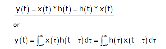
So x[t]*h[t] ⇔ h[t]*x[t]

Distributive Property

By this Property, we will conclude that convolution is distributive over addition.

• Discrete-time

x[n]{αh₁[n] + βh₂[n]} = α{x[n] h₁[n]}+ β{x[n] h₂[n]} Where, α & β are constant.

• Continuous Time

x(t){αh₁(t) + βh₂(t)} = α{x(t)h₁(t)} + β{x(t)h₂(t)} Where, α & β are constant.

Associative Property

• Discrete-Time

y[n] = x[n]*h[n]*g[n]

x[n] * h₁[n] * h₂[n] = x[n] * (h₁[n] * h₂[n])

• In Continuous Time

[x(t) * h₁(t)] * h₂(t) = x(t) * [h₁(t) * h₂(t)]

Invertibility

A system is said to be invertible if there exists an inverse system that when connected in series with the original system produces output identical to the input.

(x*δ)[n]= x[n]

(x*h*h^-1)[n]= x[n]

(h*h^-1)[n]= (δ)[n]

What is Sampling Theorem?

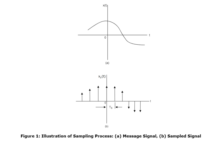
The sampling process is usually described in the time domain. In this process, an analog signal is converted into a corresponding sequence of samples that are usually spaced uniformly in time. Consider an arbitrary signal x(t) of finite energy, which is specified for all time as shown in figure 1(a).

Suppose that we sample the signal x(t) instantaneously and at a uniform rate, once every T_S second. Consequently, we obtain an infinite sequence of samples spaced T_S seconds apart and denoted by {x(nT_S)}, where n takes on all possible integer values. Thus, we can define the following terms

1. Sampling Period: The time interval between two consecutive samples is referred to as the sampling period. In the figure, T_S is the sampling period.
2. Sampling Rate: The reciprocal of the sampling period is referred to as the sampling rate, i.e. f_S = 1/T_S

The sampling theorem provides both a method of reconstruction of the original signal from the sampled values and also gives a precise upper bound on the sampling interval required for distortionless reconstruction. It states that

• A band-limited signal of finite energy, which has no frequency components higher than f Hertz, is completely described by specifying the values of the signal at instants of time separated by 1/2f seconds.
• A band-limited signal of the finite energy, which has no frequency components higher than f Hertz, may be completely recovered from a knowledge of its samples taken at the rate of 2f samples per second.

Explanation of Sampling Theorem

Consider a message signal m(t) band limited to ω, i.e.

M(f) = 0; For |f| ≥ ω

Then, the sampling frequency f_S, required to reconstruct the band-limited waveform without any error, is given by

F_s ≥ 2 ω

Aliasing and Anti-Aliasing

Aliasingsuch an effect of violating the Nyquist-Shannon sampling theory. During sampling, the baseband spectrum of the sampled signal is mirrored to every multifold sampling frequency. These mirrored spectra are called alias.

• The easiest way to prevent aliasing is the application of a steeply sloped low-pass filter with half the sampling frequency before the conversion. Aliasing can be avoided by keeping F_s > 2F_max.
• The sampling rate for an analog signal must be at least two times as high as the highest frequency in the analog signal in order to avoid aliasing. So in order to avoid this, the analog signal is then filtered by a low pass filter prior to being sampled, and this filter is called an anti-aliasing filter. Sometimes the reconstruction filter after a digital-to-analog converter is also called an anti-aliasing filter.

Nyquist Rate

Nyquist rate is defined as the minimum sampling frequency allowed to reconstruct a band-limited waveform without error, i.e.

f_N = min {f_S} = 2ω

Where,

• ω is the message signal bandwidth
• f_S is the sampling frequency.

Nyquist Interval

The reciprocal of the Nyquist rate is called the Nyquist interval (measured in seconds), i.e.

T_N = 1/f_N = 1/2W

Where,

• f_N is the Nyquist rate
• W is the message signal bandwidth.

Important GATE Notes
Astable Multivibrators	GATE Syllabus for Architecture and Planning
2’s Complement	Floating Point Representation
Cams	Statically Determinate
LU Decomposition	Connecting Rod
Infiltration Indices	Engineering Ethics
Mechanical Energy	Constant Velocity