Routing Algorithms in Computer Networs – Distance Vector, Link State

Shortest Path Routing

• Links between routers have a cost associated with them. It could be a function of distance, bandwidth, average traffic, communication cost, mean queue length, measured delay, router processing speed, etc.
• The shortest path algorithm finds the least expensive path through the network based on the cost function.
• Examples: Dijkstra’s algorithm

Distance Vector Routing

Each router periodically shares knowledge about the entire network with its neighbours in this routing scheme. Each router has a table with information about the network. These tables are updated by exchanging information with the immediate neighbours. It is also known as Belman-Ford or Ford-Fulkerson Algorithm. It is used in the original ARPANET and the Internet as RIP. 

• Neighbouring nodes in the subnet exchange their tables periodically to update each other on the state of the subnet (which makes this a dynamic algorithm). If a neighbour claims to have a path to a node shorter than your path, you start using that neighbour as the route to that node.
• Distance vector protocols (a vector contains both distance and direction), such as RIP, determine the path to remote networks using hop count as the metric. A hop count is defined as the number of times a packet needs to pass through a router to reach a remote destination.
• For IP RIP, the maximum hop is 15. Therefore, a hop count of 16 indicates an unreachable network. Two versions of RIP exist version 1 and version 2.
• IGRP is another example of a distance vector protocol with a higher hop count of 255 hops.
• Periodic updates are sent at a set interval. For IP RIP, this interval is 30 seconds.
• Updates are sent to the broadcast address 255.255.255.255. Only devices running routing algorithms listen to these updates.
• When an update is sent, the entire routing table is sent.

Link State Routing

The following sequence of steps can be executed in the Link State Routing. This advertising is a short pack called a Link State Packet (LSP). OSPF (Open shortest path first) and IS-IS are examples of Link state routing. Link State Packet(LSP) contains the following information:

1. The ID of the node that created the LSP;
2. A list of directly connected neighbours of that node, with the cost of the link to each one;
3. A sequence number;
4. A time to live(TTL) for this packet.

When a router floods the network with information about its neighbourhood, it is said to be advertising.

1. Discover your neighbours
2. Measure delay to your neighbours
3. Bundle all the information about your neighbours together
4. Send this information to all other routers in the subnet
5. Compute the shortest path to every router with the information you receive
6. Each router finds its own shortest path to the other routers using Dijkstra’s algorithm.

In link-state routing, each router shares its knowledge of its neighbourhood with all routers in the network. Link-state protocols implement an algorithm called the shortest path first (SPF, also known as Dijkstra’s Algorithm) to determine the path to a remote destination. There is no hop-count limit. (For an IP datagram, the maximum time to live ensures that loops are avoided.).Only when changes occur, It sends all summary information every 30 minutes by default. Only devices running routing algorithms listen to these updates. Updates are sent to a multicast address. As a result, updates are faster, and convergence times are reduced. Higher CPU and memory requirements to maintain link-state databases. Link-state protocols maintain three separate tables.

1. Neighbour table: It contains a list of all neighbours and the interface to which each neighbour is connected. Neighbours are formed by sending Hello packets.
2. Topology table (Link- State table): It contains a map of all links within an area, including each link’s status.
3. Routing table: It contains the best routes to each particular destination

Flooding Algorithm

It is a non-adaptive algorithm or static algorithm.  When a router receives a packet, it sends a copy of the packet out on each line (except the one on which it arrived). Each router decrements a hop count contained in the packet header to prevent looping forever.  As soon as the hop count decrements to zero, the router discards the packet.

Flow-Based Routing Algorithm

• It is a non-adaptive routing algorithm.
• It takes into account both the topology and the load in this routing algorithm;
• We can estimate the flow between all pairs of routers.
• You can compute the mean packet delays using queuing theory from the known average amount of traffic and the average length of a packet.
• Flow-based routing then seeks to find a routing table to minimize the average packet delay through the subnet.
• Given the line capacity and the flow, we can determine the delay. It needs to use the formula for delay time T.

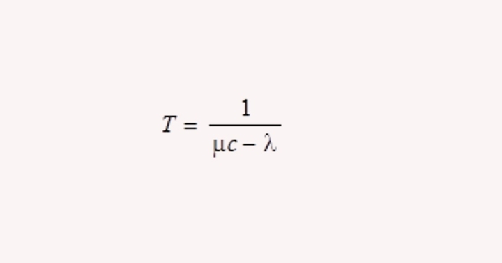
• Where, μ = Mean number of arrivals in packet/sec, 1/μ = The mean packet size in the bits, and c = Line capacity (bits/s).

Daily GATE & ESE Live Sessions, Free Live Classes, Study Notes, Quizzes & Free PDF’s & more, Join our Telegram Group.