What are Elementary Signals?

What are Elementary Signals?

Before discussing the elementary signals, we must know their significance. In any engineering application, if we want to analyze the characteristics of any system that can be a process or a physical device, we must test or analyze it with a certain set of inputs. But every time it is not possible to apply these directly to that physical device. Hence, we model the physical system into a suitable mathematical model and analyze it with a set of signals that replicate the character of the input we want to apply to this system and record its response by using various mathematical tools such as Fourier transforms, Laplace transforms, eigenfunctions, etc.

But how do we model these signals? It is not possible to model every random input, but certain sets can replicate most inputs we want to apply to the system. For example, if the nature of your input is a sudden blow in a short duration, we can model this as an impulse signal; if it is a sudden input with a finite magnitude that longs for an infinite(long) duration we can model as a step signal; if it is oscillatory, then we can model it as a sinusoidal signal. Like this, some signals those found extensive use in our applications such as

• Sinusoidal signal
• Exponential signal
• Impulse signal
• Unit step signal
• Ramp signal
• Parabolic signal

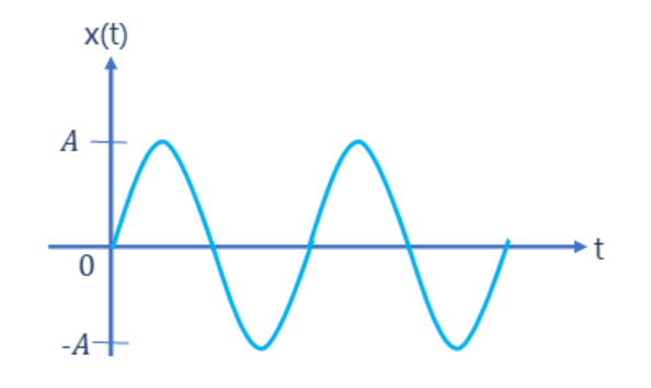
Sinusoidal Signal

The sinusoidal signal has found a versatile application in the fields like mathematics, physics, signal processing, engineering, etc, the reason behind its extensive application is that we can relate this to so many wave patterns that occur in nature like sound, wind, and the light wave. In addition to these, we can relate every physical oscillation with a sinusoidal signal. Most importantly it has a unique property that is it retains its shape when we add it with another sinusoid of the same frequency and arbitrary phase and magnitude, this property leads to the invention of the Fourier series.

its mathematical expression is

x(t)=Asin(ωt+Φ)

Where A is amplitude andΦ is phase difference.

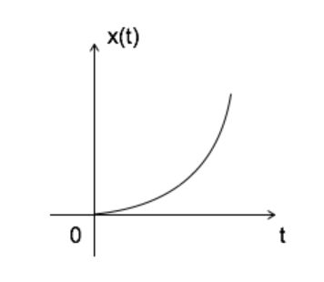
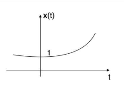
Exponential Signal

The mathematical expression for the exponential signal is given by x(t)=e^αt

The shape of this signal depends on the value of α.

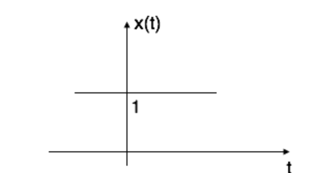
If α=0 then x(t) = e⁰ = 1

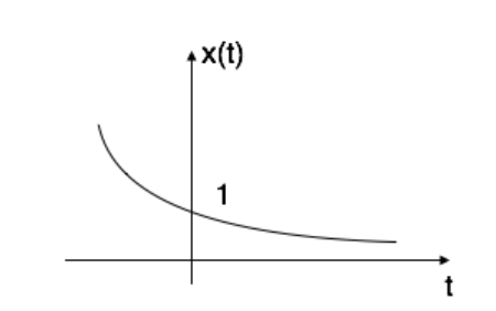
If α is less than zero, then x(t)= e^-αt, and the shape is decaying exponential.

Ifα is greater than zero then x(t)= e^αt, the shape is called raising exponentially.

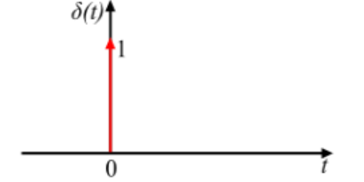
Impulse Signal

If we want to model the input of an ample magnitude that disappears in no time (very short duration) we must use the impulse signal. The ideal impulse signal is zero everywhere but infinitely high at the instant zero. But the area of the ideal impulse signal is a finite value only.

^∞∫_-∞δ(t)dt= 1

The unit impulse signal finds extensive use in the analysis of signals and systems.

The mathematical representation of continuous-time unit impulse signal is given by:

δ(t) = 1; for t = 0

andδ(t) = 0 ; for t ≠ 0

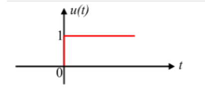
Unit Step Signal

If we want to model any signal that changes its magnitude suddenly and remains with the same magnitude for an infinite period. The mathematical expression of the unit step signal is given below.

u(t) = 1; for t≥ 0

and u(t) = 0 ; for t < 0

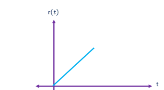
Ramp Signal

Starting at the instant t=0, the amplitude of the continuous-time ramp signal increases linearly with time. The mathematical expression of a continuous-time ramp signal is

r(t) = 1; for t≥ 0

and r(t) = 0 ; for t < 0

Ramp signal can also be expressed as r(t)= tu(t).

Parabolic Signal

The mathematical representation of the continuous-time parabolic signal is

x(t) = t²/2; for t≥ 0

and x(t) = 0 ; for t < 0