Time Domain Analysis Study notes Part-1

Time Domain Analysis

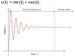
The Time Domain Analyzes of the system is to be done on basis of time. The analysis is only be applied when nature of input plus mathematical model of the control system is known. Expressing the main input signals is not an easy task and cannot be determined by simple equations. There are two components of any system’s time response, which are: Transient response & Steady state response.

Transient Response: This response is dependent upon the system poles only and not on the type of input & it is sufficient to analyze the transient response using a step input.
Steady-State Response: This response depends on system dynamics and the input quantity. It is then examined using different test signals by final value theorem.

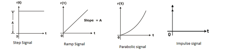
Standard Test Input Signals

Step signal: r(t) = Au(t).
Ramp signal: r(t) = At; t > 0.
Parabolic signal: r (t) At²/2; t > 0.
Impulse signal: r(t) = δ(t).

Initial value of the response [c(0)]

Initial value theorem is applied only when the number of poles of C(s) is more than the number of zeros i.e. function C(s) must be strictly proper.

Final value of the Response [c(∞)] :-

Final value theorem: - Final value theorem is applied when all the poles of S C(s) lie in the left half of the S-plane

Time-Response of First-Order System

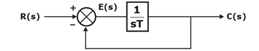
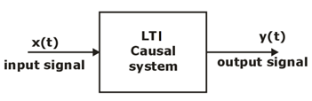
A first order control system is one for which the highest power of ‘s’ in the denominator of its transfer function is equal to 1.Thus, a first order control system is expressed by a transfer function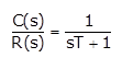

Also, the block diagram representation of the above expression is shown in the below.

Unit step input of a first order system:

The step response of a dynamic system measures how the dynamic system responds to a step input signal.

The output for the system is expressed as, C(s) = R(s)

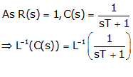
As the input is a unit step function, r(t) = 1 and R(s) = 1/s

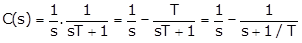
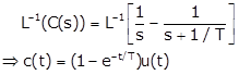
The error is given by, e(t) = r(t) – c(t) = e^–t/T. u(t)

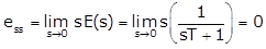
The steady state error,

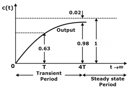
The time response in relation to above equation is shown in the figure.

Ramp response of first-order system:

As the input is a unit ramp function, r(t) = t and R(s) = 1/s²

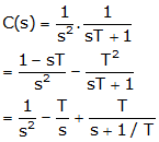
Taking inverse Laplace transform on both sides,

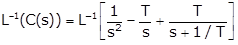
C(t) = (t – T + Te^–t/T) u(t)

The error is given by e(t) = r(t) – c(t) = (T – Te^–t/T) u(t)

The steady state error is

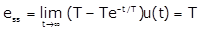
The time response in relation to the above equation is shown in the figure.

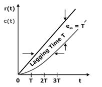
The time response shown in figure indicates that during steady state, the output velocity matches with the input velocity but lags behind the input by time T and a positional error of T units exists in the system.

Thus, the first-order system will track the unit ramp input with a steady-state error T, which is equal to the time-constant of the system.

Unit impulse response of a first order control system:

The impulse response of a dynamic system measures how the system responds to an impulse input signal.

⇒ c(t) = (1/T)e^–t/T

The error is given by e(t) = r(t) – c(t)

The steady state error is

TIME RESPONSE OF SECOND ORDER CONTROL SYSTEM

Second order systems are important for several reasons.

They are the simplest systems that exhibit oscillations and overshoot.
Many important systems exhibit second order system behavior.
Second order behavior is part of the behavior of higher order systems and understanding second order systems helps you to understand higher order systems.

A second order control system is one for which the highest power ‘s’ in the denominator of its transfer function is equal to 2.

Consider a linear time-invariant system where input to the system is given by x(t) & its corresponding output as y(t).

The general differential equation of second order system is given as

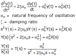is the transfer function of 2^nd order system.

The characteristic equation of the second order system is

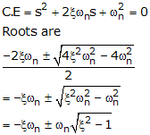
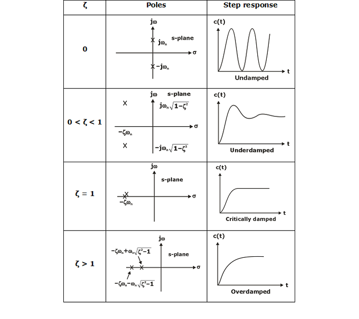
Case 1: ξ = 0

In this case, the poles of the system lie on jω axis and hence the system is said to be undamped system.

Case 2: ξ = 1

In this case, the roots or poles of the system is always real and equal and equals to –ω_n i.e. s₁, s₂ = – ω_n

Therefore, the system is said to be critically damped system.

Case 3: 0 < ξ < 1

In this case, the poles of the system are complex conjugate to each other. i.e.

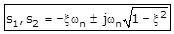
Hence, the system is called under damped system.

Case 4: ξ > 1

In this case, the roots or poles of the system are real but unequal i.e.,

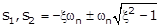
Therefore, the system is said to be over damped system.

Output Response & Pole-Zero Plot of Various Forms of Systems:

If you aiming to crack GATE & ESE, Other PSU Exams then you must try Online Classroom Program to get unlimited access to all the live structured courses and unlimited mock tests from the following links:

Time Domain Analysis Study notes Part-1