- Home/
- GATE ELECTRICAL/
- GATE EE/
- Article
Steady State Response in Control System
By BYJU'S Exam Prep
Updated on: September 25th, 2023

Steady State Response refers to the behavior of a system after it has been given enough time to stabilize in response to a constant input or disturbance. In other words, Steady state response is the behavior of a system when all the transient effects have died out, and the system has settled into a steady state. Steady-state response is characterized by the system’s output remaining constant, or oscillating at a constant frequency and amplitude.
Steady State Response GATE Notes(Download PDF)
Steady State Response is an important concept in various fields such as control theory, signal processing, and circuit analysis. In control theory, the steady-state response is used to evaluate the performance of control systems, while in signal processing, it is used to analyze the behavior of filters and other signal-processing systems. In this article, you will find the Study Notes on Steady State Response which will cover the topics such as the Response of first-order Systems, the Response of the second-order Systems, and Steady-State error.
Table of content
What is Steady State Response?
Steady state response is the behavior of a system after it has reached a stable condition in response to a constant input or disturbance. It is the response of a system when all the transient effects have died out, and the system has settled into a steady state. In other words, it is the behavior of the system over the long term, when the input or disturbance is constant or periodic.
The steady-state response of a system is characterized by the system’s output remaining constant or oscillating at a constant amplitude and frequency. The behavior of a system in a steady state is often easier to analyze and predict than its behavior during transient periods, making steady-state analysis an important tool in engineering and science.
Steady State Response is Denoted by
Many applications of control theory are to servomechanisms which are systems using the feedback principle designed so that the output will follow the input. Hence there is a need for studying the time response of the system. The time response of a system may be considered in two parts:
- Transient response: this part reduces to zero as t → ∞
- Steady-state response: response of the system as t → ∞
Response of First Order Systems
In closed-loop or open-loop control systems engineering, a first-order system is a system whose behavior can be described by a first-order differential equation. The steady-state response of a first-order system is the response that the system approaches as time goes to infinity after any transient effects have died away.
- Consider the output of a linear system in the form Y(s) = G(s)U(s) where Y(s): Laplace transform of the output, G(s): transfer function of the system, and U(s): Laplace transform of the input.
- Consider the first-order system of the form ay + y = u, its transfer function is Y(s) = U(s)/(as+1).
- For a transient response analysis, it is customary to use a reference unit step function u(t) for which U(s) = 1/s
- It then follows that Y(s) = 1/{s(as+1)} = (1/s) – (1/(s+(1/a))).
- On taking the inverse Laplace of the equation, we obtain y(t) = 1 – e-t/a
- The response has an exponential form. The constant ‘a’ is called the time constant of the system.
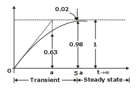
- Notice that when t = a, then y(t)= y(a)= 1- e-1=0.63. The response is in two parts, the transient response part e-t/a, which approaches zero as t →∞ and the steady-state part 1, which is the output when t → ∞.
- If the derivative of the input is involved in the differential equation of the system, that is if ay + y = bu + u then its transfer function is Y(s) = (bs+1)U(s)/(as+1) = K(s+z) U(s)/(s+p)
where,
- K = b/a
- z =1/b: the zero of the system
- p =1/a: the pole of the system
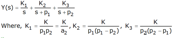
- When U(s) =1/s, Equation can be written as
![]()
- Hence, y(t) = K1 – K2e-pt
- With the assumption that z>p>0, this response is shown in
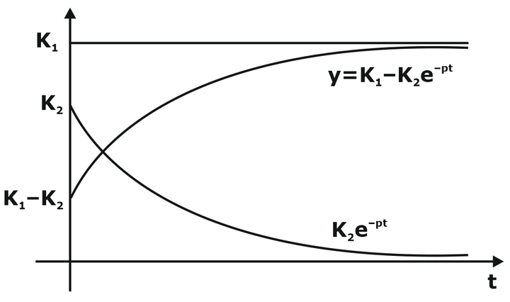
- We note that the responses to the systems have the same form, except for the constant terms K1 and K2 . It appears that the role of the numerator of the transfer function is to determine these constants, that is, the size of y(t), but its form is determined by the denominator.
Response of Second Order Systems
In control systems engineering, a second-order system is a system whose behavior can be described by a second-order differential equation. The steady-state response of a second-order system is the response that the system approaches as time goes to infinity after any transient effects have died away.
- An example of a second-order system is a spring-dash pot arrangement, Applying Newton’s law, we find M d2y/dt2 = -μ dy/dt + u(t)
- where k is the spring constant, µ is the damping coefficient, y is the distance of the system from its position of the equilibrium point, and it is assumed that y(0) = y(0)’ = 0.
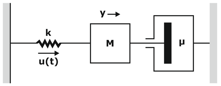
- Hence, u(t) = M d2y/dt2 + μ dy/dt + ky
- On taking Laplace transforms, we obtain,
![]()
- where K =1/ M, a1 = µ / M, a2 = k / M. Applying a unit step input, we obtain Y(s) = K/s(s+p1)(s+p2)
- where p1,2 = [a1 ± √(a12 – 4a2)]/2, p1 and p2 are the poles of the transfer function G(s) = K/(s2 + a1s + a2) that is, the zeros of the denominator of G(s).
- There are there cases to be considered:
Over Damped System
- In this case, p1 and p2 are both real and unequal. The equation can be written as
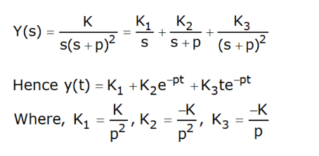
Critically Damped System
- In this case, the poles are equal: p1 = p2 = a1 / 2 = p , and
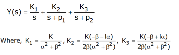
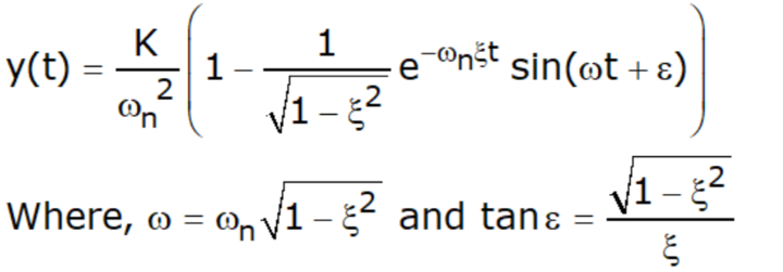
Under Damped System
- In this case, the poles p1 and p2 are complex conjugate having the form p1,2 = α±iβ where, α=a1/2 and β= 0.5 √(4a2-a12)
The three cases discussed above are plotted as:
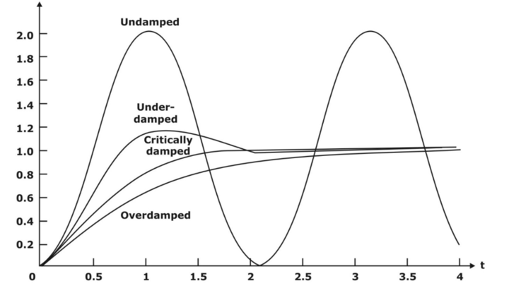
There are two important constants associated with each second-order system
- The undamped natural frequency ωn of the system is the frequency of the response shown in Fig. ωn = √a2
- The damping ratio ξ of the system is the ratio of the actual damping µ(= a1M) to the value of the damping µc, which results in the system being critically damped. Hence, ξ = μ/μc = a1/2√a2
- also,
Terminologies About Steady State Response
Here, a few terms have been explained that help to understand the concept of steady-state response in detail.
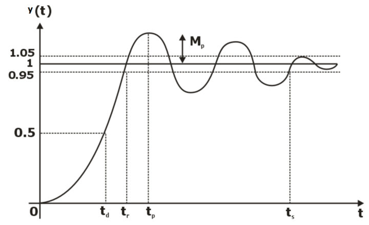
- Overshoot: It is defined as the ratio of maximum overshoot to the final desired value.
- Time delay τd: the time required for a system response to reach 50% of its final value
- Rise time: the time required for the system response to rise from 10% to 90% of its final value
- Settling time: the time required for the eventual settling down of the system response to be within (normally) 5% of its final value
- Steady-state error ess: the difference between the steady-state response and the input.
Steady State Error
Steady-state error is a term used in control theory to describe the difference between the desired output of a system and the actual output of the system once it has reached a steady-state condition. In other words, it’s the difference between the desired and actual output of a system when the input is a constant value over time.
In closed-loop control systems, the goal is to design a controller that minimizes steady-state error. A system with zero steady-state error is called a zero-error system, which means that the actual output is exactly equal to the desired output when the input is a constant value. However, in practice, it is often difficult to achieve zero steady-state error, and the goal is to minimize the error as much as possible.
Steady-state error is typically expressed as a percentage or a decimal value, and it can be calculated using mathematical formulas that depend on the specific characteristics of the system being analyzed. The steady-state error can be affected by various factors, such as the system’s gain, its time constant, and the type of input signal applied to the system.
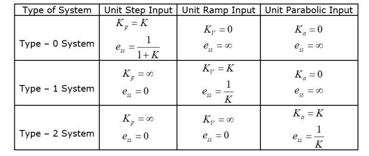
Steady-state error ess can be summarized in the below table: