Nyquist Stability Criteria & Analysis Study notes For EE/EC

Polar Plot

The polar plot of a sinusoidal transfer function G(jω) is a plot of the magnitude of G(jω) versus the phase angle of G(jω) on polar coordinates as ω varied from zero to infinity.

Procedure to Sketch the Polar Plot:

• Step-1: Determine transfer function G(jω).
• Step-2: Put s = jω in the transfer function to obtain G(jω).
• Step-3: At ω = 0 and m = ∞, calculate | G(jω)| by  and .
• Step-4: Calculate the phase angle of G(jω) at ω = 0 and ω = ∞ by  and .
• Step-5: Rationalize the function G(jω) and separate the real and imaginary axis.
• Step-6: Equate the imaginary part Im|G(jω)| to zero and determine the frequencies at which plot intersects the real axis and calculate the value of G(jω) at the point of intersection by substituting the determined value of frequency in the expression of G(jω).
• Step-7: Equate the real part Re|G(jω)| to zero and determine the frequencies at which plots intersects the imaginary axis and calculate the value G(jω) at the point of intersection by substituting the determined value of frequency in the rationalized expression of G(jω).
• Step-8: Sketch the polar plot with the help of above information.

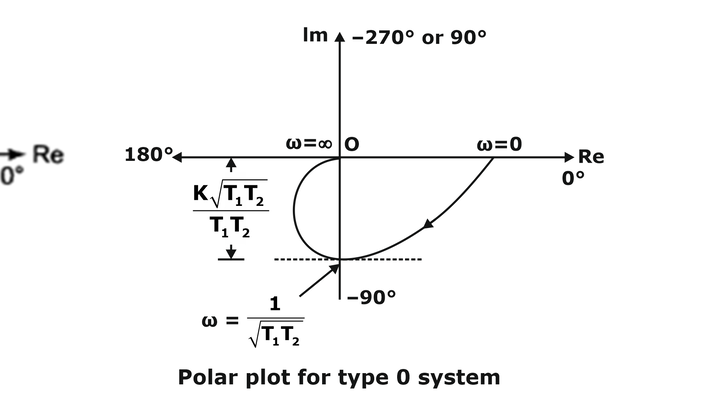
Polar Plot of Some Standard Functions:

• Type 0 System 

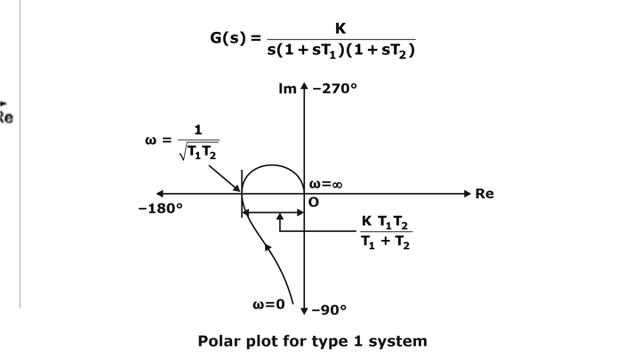
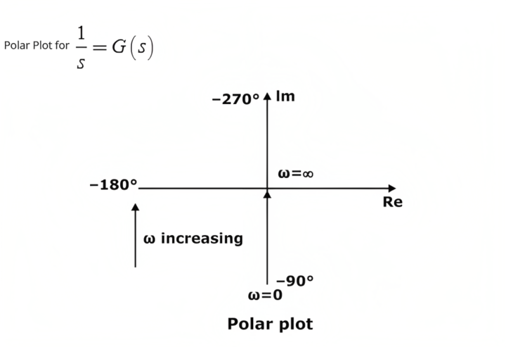
• Type 1 System

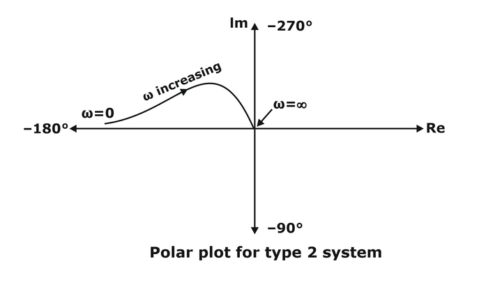
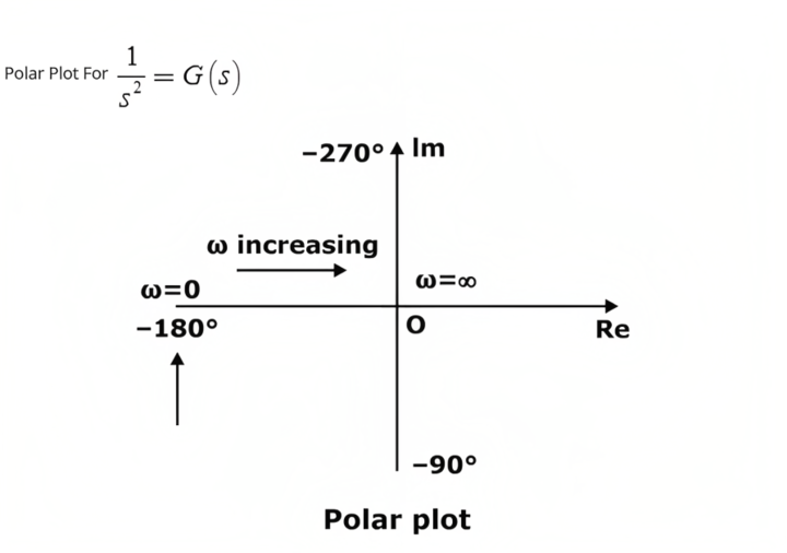
• Type 2 System

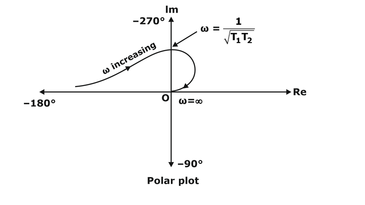
Introduction of Additional Pole

Polar Plot for 

Polar Plot For 

Gain Margin and Phase Margin with Polar Plot

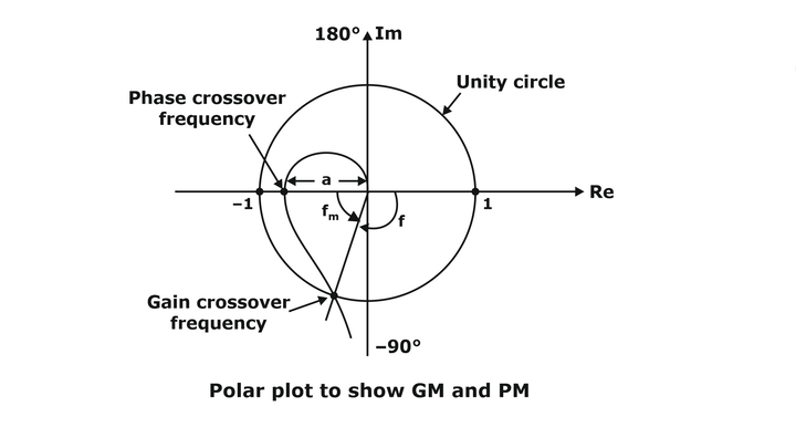
• Phase Crossover Frequency: The frequency at which the polar plot crosses the -180° line is called phase crossover frequency.
• Gain Crossover Frequency: The frequency at which the polar plot crosses the unity circle is called gain crossover frequency.
• Gain Margin: At phase crossover frequency, if gain is 'a' then

Gain margin = - 20 log a

• Phase Margin (φ_m): At gain crossover frequency, if phase is φ then phase margin

φ_m = 180 + φ

       where, φ is positive from anti-clockwise direction.

Nyquist Stability Criterion

A stability test for time invariant linear systems can also be derived in the frequency domain. It is known as Nyquist stability criterion. It is based on the complex analysis result known as Cauchy’s principle of argument.Nyquist criterion is used to identify the presence of roots of a characteristic equation of a control system in a specified region of s-plane. Nyquist approach is same as Routh-Hurwitz but, it differ with following aspect

• The open loop transfer function "G(s)H(s)" is considered instead of closed loop characteristic equation " 1+G(s) H(s) = 0".
• Inspection of graphical plot of G(s) H(s) enables to get more than yes or no answer of Routh-Hurwitz method pertaining to stability of control system.
• Nyquist plots display both amplitude and phase angle on a single plot, using frequency as a parameter in the plot.
• Nyquist plots have properties that allow you to see whether a system is stable or unstable. It will take some mathematical development to see that, but it's the most useful property of Nyquist plots.

Concept of Encirclement & Enclosement

Encirclement:

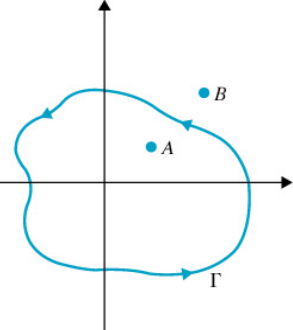
• point A is encircled in the counter in Counter Clock Wise by closed path, while point B is NOT encircled by closed path.

Enclosement: A point or region is said to be enclosed by a closed path if the point or region lies to the right of the path when the path is traversed in any prescribed direction.

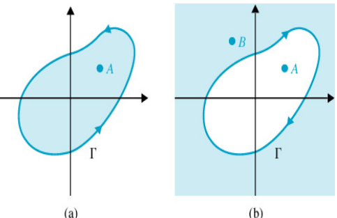
• In figure (a) point A is not enclosed by Path,while Point B is enclosed by path.
• In figure (b) point A is enclosed by Path, while point B is not enclosed by path.

Nyquist Stability Criterion : Fundamentals

Consider the phasor from point A to S₁ of encirclement = N, the net angle traversed by the phasor = 2πN rad

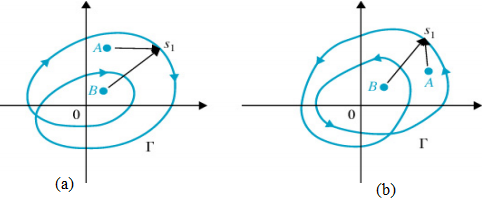
• In figure (a) Point A of encirclement = +1; Point B of encirclement = +2.
• In figure (b) Point A of encirclement = -1; Point B of encirclement = -2.

Determination of N:

• For a SISO feedback system the closed-loop transfer function is given by

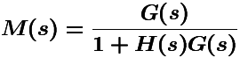
• closed-loop system poles are obtained by solving the following equation

       1+G(s)H(s) =0 =Δ(s) represents the system characteristic equation.

• In the following we consider the complex function

D(s) = 1+G(s)H(s)

• The zeros of D(s) are the closed-loop poles of the transfer function. Here now we concluded that the poles of D(s) are the zeros of M(s).
• At the same time the poles  of D(s) are the open-loop control system poles since they are contributed by the poles of H(s)G(s), which can be considered as the open-loop control system transfer function—obtained when the feedback loop is open at some point.
• The Nyquist stability test is obtained by applying the Cauchy principle of argument to the complex function D(s).First,we state Cauchy’s principle of argument.

Cauchy’s Principle of Argument

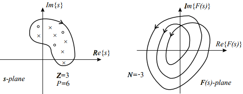
• Let F(s) be an analytic function in a closed region of the complex s-plane, except at a finite number of points (namely,the poles of F(s)).
• It is also assumed that F(s) is analytic at every point on the contour. Then, as 's' travels around the contour in the s-plane in the clockwise direction, the function F(s) encircles the origin in the [ReF{(s)},Img{F(s)}]-plane in the same direction N times , where N given By

N= P-Z

       where Z and P stand for the number of zeros and poles (including their multiplicities) of the function F(s) inside the contour.

• The above result can be also written as 

arg{F(s)} = (Z-P)2π = 2Nπ

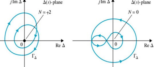
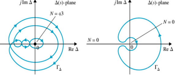
Nyquist Plot

The Nyquist plot is a polar plot of the function D(s) = 1+ G(s)H(s) when travels around the contour

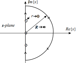
• The contour in the above figure covers the whole unstable half plane of the complex plane s, R→∞.
• Since the function D(s), according to Cauchy’s principle of argument, must be analytic at every point on the contour, the poles D(s) of on the imaginary axis must be encircled by
  infinitesimally small semicircles.

Nyquist Criterion: 

• It states that the number of unstable closed-loop poles is equal to the number of unstable open-loop poles plus the number of encirclements of the origin of the Nyquist plot of the complex function F(s).
• The above criterion can be slightly simplified if instead of plotting the function "D(s) = 1+G(s)H(s)", we plot only the function G(s)H(s) and count encirclement of the Nyquist plot of G(s)H(s) around the point (-1+j0). 
• The number of unstable closed-loop poles (Z) is equal to the number of unstable open-loop poles (P) plus the number of encirclements (N) of the point (-1+j0) of the Nyquist plot of G(s)H(s), that is

Z= P+N

Phase and Gain Stability Margins

Two important notions can be derived from the Nyquist diagram: phase and gain stability margins. The phase and gain stability margins are presented in Figure below

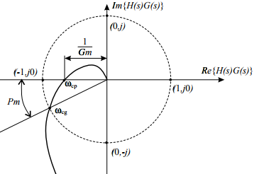
• They give the degree of relative stability; in other words, they tell how far the given system is from the instability region. Their formal definitions are given by

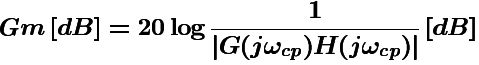
• where ω_gc and ω_pc stand for, respectively, the gain and phase crossover frequencies, which are obtained from the figure as 

Example: Consider a control system represented by

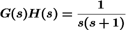
Solution: Since this system has a pole at the origin, the contour in the -plane should encircle it with a semicircle of an infinitesimally small radius. This contour has three parts (a), (b), and (c). Mappings for each of them are considered below.

•  On this semicircle the complex variable 's' is represented in the polar form by 's = Re^jψ' with R→∞, - π/2 ≤ ψ ≥ π/2. Substituting 's = Re^jψ' into G(s)H(s), we easily see that G(s)H(s)→0 . Thus, the huge semicircle from the -plane maps into the origin in the -plane .

         Thus, the huge semicircle from the s-plane maps into the origin in the G(s)H(s)-plane.

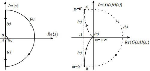
• On this semicircle the complex variable is represented in the polar form by  's = re^jψ' with r→0, - π/2 ≤ ψ ≥ π/2. so that we have

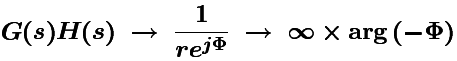
     Since φ changes from  '- π/2' at point A to ' π/2' at point B, arg{G(s)H(s)} will change from "π/2 to -π/2"  . We conclude that the infinitesimally small semicircle at the origin in the      s-plane is mapped into a semicircle of infinite radius in the G(s)H(s)-plane.

• On this part of the contour s takes pure imaginary values, i.e.  s= jω with ω  changing  from'-∞ to +∞'.Due to symmetry, it is sufficient to study only mapping along "0⁺≤ ω ≥+∞" . We can find the real and imaginary parts of the function G(jω)H(jω), which are given by

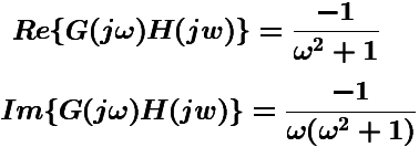
From the above expressions, we see that neither the real nor the imaginary parts can be made zero, and hence the Nyquist plot has no points of intersection with the coordinate axis. For ω= 0⁺ we are at point B and since the plot at  ω= +∞ will end up at the origin.Note that the vertical asymptote of the Nyquist plot is given by

{Re G(jo±)H(jo±)} = -1

• From the Nyquist diagram we see that N= 0 and since there are no open-loop poles in the left half of the complex plane, i .e.P=0, we have Z =0 so that the corresponding closed-loop system has no unstable poles.

If you aiming to crack GATE & ESE, Other PSU Exams then you must try Online Classroom Program to get unlimited access to all the live structured courses and unlimited mock tests from the following links:

ESE and GATE EC Online Classroom Program (24+ LIVE Courses and 150+ Mock Tests)

ESE and GATE EE Online Classroom Program (24+ LIVE Courses and 193+ Mock Tests)

Click on the Links Below to Avail Test Series:

Click Here Avail GATE/ESE EC Test Series !!! (150+ Mock Tests)

Click Here Avail GATE/ESE EE Test Series !!! (193+ Mock Tests)

Thanks