- Home/
- GATE ELECTRICAL/
- GATE EE/
- Article
Routh-Hurwitz and Various Plots (Bode Plot) Study notes For EE/EC
By BYJU'S Exam Prep
Updated on: September 25th, 2023

We will explore the Routh-Hurwitz stability criterion, a powerful tool used to determine the stability of linear time-invariant systems. Understanding stability is crucial in designing robust control systems, and the Routh-Hurwitz method offers an efficient and systematic approach to analysing the stability of complex systems. We will cover the step-by-step procedure for constructing the Routh array and determining the number of poles in the left-half plane, providing you with a solid foundation to assess system stability in various engineering applications.
Moving on to the second part, our focus will be on Bode Plot analysis. Bode Plots are graphical representations of a system’s frequency response, providing insights into its magnitude and phase characteristics. We will learn how to create Bode Plots for both open-loop and closed-loop systems, interpreting the plots to analyze the system’s stability, gain margin, and phase margin. Additionally, you will discover how to design controllers using Bode Plots to achieve desired system performance. Whether you are an electrical or electronics engineering student or a professional seeking to strengthen your skills, these study notes will equip you with the necessary knowledge to tackle real-world challenges in control systems and circuit design.
Download Formulas for GATE Electrical Engineering – Electrical Machines
Table of content
Routh-Hurwitz Stability Criterion
The technique Routh-Hurwitz criterion is a method to know whether a linear system is stable or not by examining the locations of the roots of the characteristic equation. The method determines only if there are roots that lie outside of the left half of s plane; while it does not actually compute the location of roots.
Here we have a Transfer Function F(s):
![]()
where N(s) & D(s) are the Polynomials in s. for Poles (equating D(s)= 0) & for Zeros (equating N(s)=0).
The Characteristic Equation of the above Transfer Function can be written as
1+G(s)H(s) = 0 ; or D(s)= a0sn+a1sn-1 + ……..an-1s + an = 0
To find out whether the system is stable or not, check the following conditions:
1. Two necessary but not sufficient conditions that all the roots have negative real parts.
- All the polynomial coefficients must have the same sign.
- All the polynomial coefficients must be non-zero.
2. If condition (1) is satisfied, then compute the Routh-Hurwitz array as follows
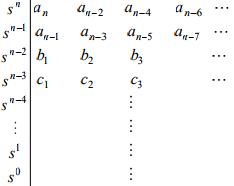
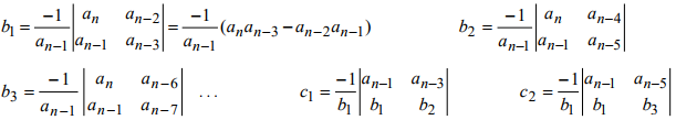
- where the ai are the polynomial coefficients, these coefficients in the rest of the table are computed as follows:
- The necessary condition for stability is that all roots must have negative real parts for this all the elements in the first column of the array have the same sign.
- The number of sign changes equals to the number of roots with positive real parts.
Special Case-1: If the first Element in a row is zero
- If the first element of a row is zero, but some other elements in that row are non-zero. Here we can replace the zero element with ε, & complete the table, and then interpret the results assuming that ε is a small number of the same sign as the element above it. The results must be interpreted in the limit as ε→0
Special Case-2: If Complete Row is zero
- Whenever all the coefficients in a row are zero, this indicates a pair of roots of equal magnitude and opposite sign.
- Here the Possibilities of these two roots could be on the Real or Imaginary axis with equal magnitudes and opposite signs.
- The zero row is replaced by taking the coefficients of dP(s)/ds, where P(s), called the auxiliary polynomial, is obtained from the values in the row above the zero row. The pair of roots can be found by solving dP(s)/ds = 0.
- It is to be noted that the auxiliary polynomial always has an even degree.
Example: Use of Auxiliary Polynomial
Consider the characteristics equation A(s) = 0
where A(s) is s5+2s4+24s3+48s2-25s-50=0
Solution: The Routh array starts off as
![]()
The auxiliary polynomial P(s) will be
P(s) = 2s4 + 48s2 − 50
which shows that A(s) = 0 must have two pairs of roots of equal magnitude and opposite sign, which are also roots of the auxiliary polynomial equation P(s) = 0.
Considering the derivative of P(s) with respect to s we get ⇒ dP(s)/ds = 8s3 + 96s.
so the s3 row is as shown below and the Routh array will be
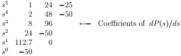
- Now there is a single change of sign in the first column of the resulting array, indicating that A(s) = 0 has one pair of symmetric roots. this symmetric root could be on a real or imaginary axis.
On Solving the Auxiliary Polynomial 2s4 + 48s2 − 50 = 0 it yields the remaining roots such as
- s2 = 1 ⇒ s= ±1
- s2 = -25 ⇒ s = ± j5
- so the original equation can be factored as ⇒ (s + 1)(s − 1)(s + j5)(s − j5)(s + 2) = 0.
Relative Stability Analysis
- Routh’s stability criterion provides the answer to the question of absolute stability. This, in many practical cases, is not sufficient. We usually require information about the relative stability of the system.
- A real approach to examine relative stability is to shift the s-plane, here we substitute s = z − σ (σ = constant) into the characteristic equation, write the polynomial in terms of z, and then apply Routh’s stability criterion to the new polynomial in z.
- The number of changes of sign in the first column of the array of Polynomial in z is equal to the number of roots which are located to the right of the vertical line s =−σ. Thus, this test reveals the number of roots which lie to the right of the vertical line s = −σ.
Root-Locus Technique
The Root Locus plots are a very useful way to predict the behaviour of a closed loop system as some parameter of the system (typically a gain) is changed. Here we will show how to draw root locus plots.
- Consider a closed-loop system with unity feedback that uses simple proportional controller.
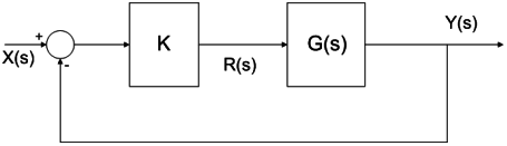
It has a transfer function
![]()
- The poles are the roots of D(s) & are obtained from the denominator of the system transfer function ⇒ 1 + KG(s) = 0, this equation is called the Characteristic equation of the system.
- Therefore it is necessary that
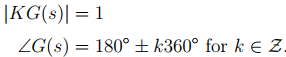
- These above two conditions are referred to as the Magnitude and Angle criteria respectively.
Effects of Addition of Poles: The effects of the addition of poles are as follows
- There is a change in the shape of the root locus and it shifts towards the imaginary axis. The intercept on the jω axis occurs for a lower value of K because of the asymptote angle being lower down.
- The system becomes oscillatory.
- Gain margin and relative stability decrease.
- There is a reduction in the range of K.
- A sluggish response can be changed to a quicker response for the artful introduction of a pole.
- Settling time increases.
Effects of Addition of Zeros: The effects of the addition of zeros are as follows
- There is a change in the shape of the root locus and it shifts towards the left of the s-plane.
- The stability of the system is enhanced.
- Range of K increases.
- Settling time speeds up.
Bode Plot
The bode plot gives a graphical method for determining the stability of a control system based on sinusoidal frequency response. Bode graphs are representations of the magnitude and phase of G(jω) (where the frequency ω contains only positive frequencies).
The bode plot consists of two graphs: Magnitude plot and Phase plot
- 20 log10 |G (jω)| versus logω, this is called a magnitude plot.
- Phase shift (in degrees) versus logω (frequency), is called a phase plot.
- Bode plots are asymptotic log magnitude and phase plots. These are drawn as straight lines.
- The corner frequency is the frequency at which the slope of the asymptotic log magnitude plot changes.
- The frequency band from ω1 and ω2 such that (ω2/ω1) = 10 is called a decade.
- For a first-order factor, the slope of the Log magnitude plot changes by ±20 dB/decade at the corner frequency according to the factor in the numerator or denominator respectively. For a second-order factor, the slope changes by ±40 dB/decade and so on.
Initial Slope of the Bode Plot: Initial slope can be determined by the type of the system, Its value is different for different types of systems.
- Type 0 system: For this system, the initial slope is 0 dB/decade with a dB value of 20 log K.
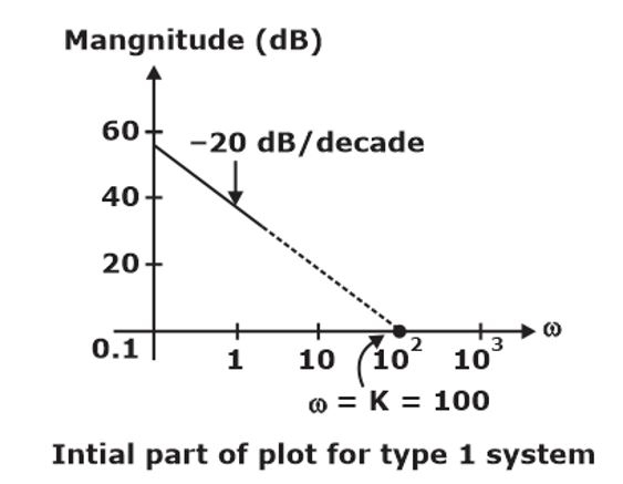
- Type 1 system: For this system, the initial part of the system is

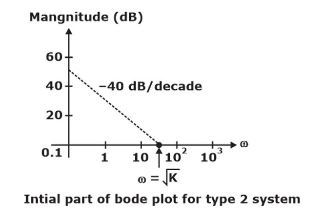
- Type 2 system: For type 2 system, initial part of plot is
![]()
Here, the initial slope is -40 dB/decade and plot cuts the 0 dB line at ![]()
Phase Margin and Gain Margin
The PM and GM can be calculated by considering the following plot
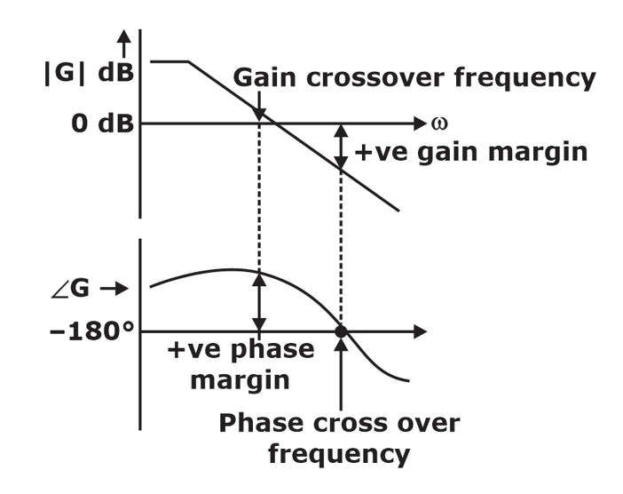
- Gain Crossover Frequency: Frequency at which magnitude plot crosses the 0 dB line.
- Phase Crossover Frequency: Frequency at which phase plot crosses the -180° line.
- Gain Margin: The value of gain from the gain plot at phase crossover frequency is called the gain margin. The gain margin is positive if it is below from zero dB line.
- Phase Margin: The value of phase from phase plot at the gain crossover frequency is known as phase margin. The phase margin is positive if it is above from -180° line.
Minimum Phase, Non-minimum Phase and All-Pass Transfer Function
- Minimum phase transfer function:
![]()
- Non-minimum phase system:
![]()
- All pass transfer functions:
![]()
- If there are no poles of the transfer function at the origin, the initial slope of the Bode magnitude plot is zero and the magnitude is 20 log K up to the lowest corner frequency.
- If there is a single pole at the origin in the open loop transfer function the Bode magnitude plot has an initial slope equal to -20 dB/decade up to the lowest corner frequency and if this line is extended, it will intersect the frequency axis at ω = kv.
- If there are two poles at the origin in the open loop transfer function, the Bode magnitude plot has an initial slope equal to -40 dB/decade up to the lowest corner frequency and this line is extended will intersect the frequency axis at
 .
. - If there is one zero at the origin, the Bode magnitude plot has an initial slope equal to 20 dB/decade up to the lowest corner frequency. If there are two zeros at the origin, the Bode magnitude plot has an initial slope equal to +40 dB/decade up to the lowest corner frequency and so on.
- Multiplication of the transfer function by a gain factor is equivalent to shifting the Bode magnitude plot vertically up by an equivalent gain in dB.
If you aiming to crack GATE & ESE, Other PSU Exams then you must try Online Classroom Program to get unlimited access to all the live structured courses and unlimited mock tests from the following links:
ESE and GATE EC Online Classroom Program (24+ LIVE Courses and 150+ Mock Tests)
ESE and GATE EE Online Classroom Program (24+ LIVE Courses and 193+ Mock Tests)
Click on the Links Below to Avail Test Series:
Click Here to Avail GATE/ESE EC Test Series !!! (150+ Mock Tests)
Click Here to Avail GATE/ESE EE Test Series !!! (193+ Mock Tests)
Get complete information about the GATE exam pattern, cut-off, and all those related things on the BYJU’S Exam Prep official youtube channel.