Control Systems - Frequency Domain Analysis Complete Study Notes

In a feedback control system, at least part of the information used to change the output variable is derived from measurements performed on the output variable itself. This type of closed-loop control is often used in preference to open-loop control (where the system does not use output-variable information to influence its output) since feedback can reduce the sensitivity of the system to externally applied disturbances and to changes in system parameters.
Familiar examples of feedback control systems include residential heating systems, most high-fidelity audio amplifiers, and the iris-retina combination that regulates light entering the eye.

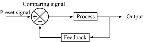
Closed-loop control system:

Sometimes, we may use the output of the control system to adjust the input signal. This is called feedback. Feedback is a special feature of a closed-loop control system.
A closed-loop control system compares the output with the expected result or command status, then it takes appropriate control actions to adjust the input signal.
Therefore, a closed-loop system is always equipped with a sensor, which is used to monitor the output and compare it with the expected result.

The following figure shows a simple closed-loop system.

The output signal is feedback to the input to produce a new output.
A well-designed feedback system can often increase the accuracy of the output.

Block diagram of a closed-loop control system

Feedback can be divided into positive feedback and negative feedback.

Positive Feedback:

Positive feedback causes the new output to deviate from the present command status.
For example, an amplifier is put next to a microphone, so the input volume will keep increasing, resulting in a very high output volume.

Negative Feedback:

Negative feedback directs the new output towards the present command status, so as to allow more sophisticated control.
For example, a driver has to steer continuously to keep his car on the right track.

Most modern appliances and machinery are equipped with closed-loop control systems. Examples include air conditioners, refrigerators, automatic rice cookers, automatic ticketing machines, etc. An air conditioner, for example, uses a thermostat to detect the temperature and control the operation of its electrical parts to keep the room temperature at a preset constant.

Block diagram of the control system of an air conditioner

One advantage of using the closed-loop control system is that it is able to adjust its output automatically by feeding the output signal back to the input.
When the load changes, the error signals generated by the system will adjust the output. However, closed-loop control systems are generally more complicated and thus more expensive to make.
Feedback is a common and powerful tool when designing a control system.
The feedback loop is the tool that takes the system output into consideration and enables the system to adjust its performance to meet a desired result of the system.

In any control system, the output is affected due to a change in environmental conditions or any kind of disturbance. So one signal is taken from the output and is fed back to the input. This signal is compared with reference input and then an error signal is generated. This error signal is applied to the controller and output is corrected. Such a system is called a feedback system.

When the feedback signal is positive then the system called a positive feedback system. For a positive feedback system, the error signal is the addition of reference input signal and the feedback signal.
When the feedback signal is negative then the system is called a negative feedback system. For a negative feedback system, the error signal is given by the difference of reference input signal and the feedback signal.

Feedback characteristics: Including feedback into the control of a system results in the following.

Advantages:

Increased accuracy. The output can be made to reproduce the input
Reduced sensitivity to system characteristics
Reduction in the effect of non-linearities
Increased bandwidth. The system can be made to respond to a larger range of input frequencies.

The major disadvantages resulting from feedback are the increased risk of instability and the additional cost of design and implementation.

Applications of Feedback: Flight control systems, Robotics, Chemical process control, Communications & Networks, Automotive, Biological Systems, Environmental Systems & Quantum Systems.

Rule to Draw the Root Locus Plot

Rule 1-Symmetry: Since the characteristic equation has real coefficients, any zeros must occur in complex conjugate pairs (which are symmetric about the real axis). Since the root locus is just a diagram of the roots of the characteristic equation as K varies, it must also be symmetric about the real axis.

Rule 2-Number of Branches: Since the order of the characteristic equation is the same as that of the denominator of the loop gain, the number of branches is n, the order of the denominator polynomial.

Rule 3- Starting and Ending Points: Start from the magnitude condition: K|N(s)/D(s)| =1

So the locus starts (when K=0) at poles of the loop gain, and ends (when K→∞) at the zeros. Note: there are q zeros of the loop gain as s→∞.

Rule 4- Locus On The Real Axis: The locus exists on the real axis to the left of a sum of the number of poles and zeros is odd on the axis.

Rule 5- Number of Branches Terminating to Infinity: If for a given system the number of Open Loop Poles are P & the number of Open Loop Zeros are Z then there will be "P-Z" branches which are terminating to Infinity.

Rule 6- Asymptotes Angle & Centroid: We know that if we have a characteristic equation P(s) that has more poles (P=N) than zeros (Z=M) then "N−M" of the root locus branches tend to zeros at infinity.

These asymptotes intercept the real axis at a point, Called it Centroid σ_A,

Or in other words

The angles of the asymptotes φ_k are given by for K>0

where, q = 0, 1, 2, ..., n – m – 1.

The angles of the asymptotes φ_k are given by for K<0

where, q = 0, 1, 2, ..., n – m – 1.

Rule 7-Determining the Breakaway Points:

First of all, we have to identify the portions of the real axis where a breakaway point must exist.
Assuming we have already marked the segments of the real axis that are on the root locus, we need to find the segments that are the part of the root locus by either two poles or two zeros (either finite zeros or zeros at infinity).
To estimate the values of s at the breakaway points, the characteristic equation ⇒
1 + KP(s) = 0 is rewritten in terms of K as

To find the breakaway points we find the values of s corresponding to the maxima in K(s). i.e. where dK/ds = K'(s) = 0.

As the last step, we check the roots of K'(s) that lie on the real axis segments of the locus. The roots that lie in these intervals are the breakaway points.

Rule 8- Find the angles of departure/arrival for complex poles/zeros:

The angle of departure (θ_d) is given by θ_d = 180° + arg [G(s )H(s ) where arg [G(s )H(s)] is the angle of G(s)H(s) excluding the pole where the angle is to be calculated.
Similarly, the angle of arrival is given by θ_a = 180° - arg [G(s)H(s)], where arg [G(s)H(s)] is the angle of G(s)H(s) excluding the zero, where the angle is to be calculated.
When there are complex poles or zeros of P(s), the root locus branches will either depart or arrive at an angle θ where, for a complex pole or zero at s = p or s = z,

where

In other words

Therefore, exploiting the rules of complex numbers, we can rewrite ∠P^∗(p)and ∠P^∗(z) as

Rule 9- Intersection of the Root Locus with the jω Axis: To find the intersection of root locus with the imaginary axis. The following procedures are followed

Step 1: Construct the characteristic equation 1+ G(s) H(s) = 0

Step 2: Develop Routh array in terms of K.

Step 3: Find K_mar that creates one of the roots of the Routh array as a row of zeros.

Step 4: Frame auxiliary equation A(s) = 0 with the help of the coefficient of a row just above the row of zeros.

Step 5: The roots of the auxiliary equation A(s) = 0 for K = K_mar give the intersection points of the root locus with the imaginary axis.

Value Gain Margin:

Grain Margin (GM) =

Note: If the root locus does not cross the jω axis, the gain is ∞. GM represents the maximum gain that can be multiplied for the system to be just on the verge of instability.

Phase Margin: Phase margin (PM) can be determined for a given value of K as follows

Calculate ω for which |G (jω) H (jω)| = 1 for the given value of K.
Calculate [G (jω) H (jω)]
Phase margin = 180° + arg [G (jω) H (jω)]

Routh-Hurwitz Stability Criterion

The technique Routh-Hurwitz criterion is a method to know whether a linear system is stable or not by examining the locations of the roots of the characteristic equation. The method determines only if there are roots that lie outside of the left half-plane; while it does not actually compute the roots.

Here we have a Transfer Function F(s):

where N(s) & D(s) are the Polynomials in s to know the Poles (by equating D(s)= 0) & Zeros (by equating N(s)=0).

The Characteristic Equation of the above Transfer Function can be written as

1+G(s)H(s) = 0 ; or D(s)= a_nsⁿ+a_n-1s^n-1 + ........a₁s + a_o =0

To find out whether the system is stable or not, check the following conditions:

1. Two necessary but not sufficient conditions that all the roots have negative real parts are

All the polynomial coefficients must have the same sign.
All the polynomial coefficients must be non-zero.

2. If condition (1) is satisfied, then compute the Routh-Hurwitz array as follows

where the a_i are the polynomial coefficients, these coefficients in the rest of the table are computed as follow:

The necessary condition that all roots have negative real parts is that all the elements of the first column of the array have the same sign.
The number of changes of sign equals the number of roots with positive real parts.

Special Case-1: Zero First-Column Element

If the first element of a row is zero, but some other elements in that row are nonzero. Here we can replace the zero elements with "ε", & complete the table, and then interpret the results assuming that "ε" is a small number of the same sign as the element above it. The results must be interpreted in the limit as ε→0

Special Case-2: If Complete Zero Row.

Whenever all the coefficients in a row are zero, a pair of roots of equal magnitude and the opposite sign will be present.
Here the Possibilities of these two roots could be Real or Conjugate Imaginary with equal magnitudes and opposite signs.
The zero row is replaced by taking the coefficients of dP(s)/ds, where P(s), called the auxiliary polynomial, is obtained from the values in the row above the zero row. The pair of roots can be found by solving dP(s)/ds = 0.
It is to be noted that the auxiliary polynomial always has even degree.

Example: Use of Auxiliary Polynomial

Consider the quintic equation A(s) = 0 where A(s) is

s⁵+2s⁴+24s³+48s²-50=0

Solution: The Routh array starts off as

The auxiliary polynomial P(s) will be

P(s) = 2s⁴ + 48s² − 50

which shows that A(s) = 0 must have two pairs of roots of equal magnitude and opposite sign, which are also roots of the auxiliary polynomial equation P(s) = 0.

Considering derivative of P(s) with respect to s we get ⇒ dP(s)/ds = 8s³ + 96s.

so the s³ row is as shown below and the Routh array will be

Now there is a single change of sign in the first column of the resulting array, indicating that there A(s) = 0 has one root with a positive real part.

On Solving the Auxiliary Polynomial 2s⁴ + 48s² − 50 = 0 it yields the remaining roots such as

s² = 1 ⇒ s= ±1
s² = -25 ⇒ s = ± j5
so the original equation can be factored as ⇒ (s + 1)(s − 1)(s + j5)(s − j5)(s + 2) = 0.

Relative Stability Analysis

The Routh’s stability criterion provides the answer to the question of absolute stability. This, in many practical cases, is not sufficient. We usually require information about the relative stability of the system.
A real approach to examine relative stability is to shift the s-plane, here we substitute s = z − σ (σ = constant) into the characteristic equation, write the polynomial in terms of z and then apply Routh’s stability criterion to the new polynomial in z.
The number of changes of sign in the first column of the array of Polynomial in z is equal to the number of roots which are located to the right of the vertical line s =−σ. Thus, this test reveals the number of roots which lie to the right of the vertical line s = −σ²